Mesh adaptation
From CFD-Wiki
m |
(→r-Refinement: Added sketch) |
||
| (9 intermediate revisions not shown) | |||
| Line 1: | Line 1: | ||
| - | + | {{Meshing table of contents}} | |
| - | + | [[Unstructured mesh generation|<< Unstructured Mesh Generation]] | '''Mesh Adaptation''' | [[ First cell height calculation|First cell height calculation>>]] | |
| - | Mesh adaptation | + | Mesh adaptation, often referred to as Adaptive Mesh Refinement (AMR), refers to the modification of an existing mesh so as to accurately capture flow features. Generally, the goal of these modifications is to improve resolution of flow features without excessive increase in computational effort. We shall discuss in brief on some of the concepts important in mesh adaptation. |
| - | + | Mesh adaptation strategies can usually be classified as one of three general types: r-refinement, h-refinement, or p-refinement. Combinations of these are also possible, for example hp-refinement and hr-refinement. We summarise these types of refinement below. | |
| - | + | ==r-Refinement== | |
| + | r-refinement is the modification of mesh resolution without changing the number of nodes or cells present in a mesh or the connectivity of a mesh. The increase in resolution is made by moving the grid points into regions of activity, which results in a greater clustering of points in those regions. The movement of the nodes can be controlled in various ways. On common technique is to treat the mesh as if it is an elastic solid and solve a system equations (suject to some forcing) that deforms the original mesh (see for instance [http://en.wikipedia.org/wiki/Stretched_grid_method Stretched grid method]). Care must be taken, however, that no problems due to excessive grid skewness arise. | ||
| - | + | [[File:Mesh_R-Refinement.png]] | |
| - | + | ==h-Refinement== | |
| + | h-refinement is the modification of mesh resolution by changing the mesh connectivity. Depending upon the technique used, this may not result in a change in the overall number of grid cells or grid points. The simplest strategy for this type of refinement subdivides cells, while more complex procedures may insert or remove nodes (or cells) to change the overall mesh topology. | ||
| - | + | In the subdivision case, every "parent cell" is divided into "child cells". The choice of which cells are to be divided is addressed below. For every parent cell, a new point is added on each face. For 2-D quadrilaterals, a new point is added at the cell centroid also. On joining these points, we get 4 new "child cells". Thus, every quad parent gives rise to four new offsprings. The advantage of such a procedure is that the overall mesh topology remains the same (with the child cells taking the place of the parent cell in the connectivity arrangement). The subdivision process is similar for a triangular parent cell, as shown below. It is easy to see that the subdivision process increases both the number of points and the number of cells. | |
| - | + | [[Image:MESH_subdivide.png]] | |
| - | + | An additional point to be noted is that this type of mesh adaptation can lead to what are called "hanging nodes." In 2D, this happens when one of the cells sharing a face is divided and the other is not, as shown below. For two quad cells, one cell is divided into four quads and other remains as it is. The highlighted node is the hanging node. | |
| - | Just as refinement is possible by ERROR INDICATORS as mentioned above, certain other issues also assume relevance. Error Indicators do detect regions for refinement, they do not actually tell if the resolution is good enough at any given time. In fact the issue is very severe for shocks, the smaller the cell, the higher the gradient and the | + | [[Image:MESH_hanging.png]] |
| + | |||
| + | This leads to a node on the face between the two cells which does not belong (properly) to both of the cells. The node "hangs" on the face, and one of the cells becomes an arbitrary polyhedron. In the above case, the topology seemingly remains same, but the right (undivided) cell actually has five faces. | ||
| + | |||
| + | Further, there are two ways of h-refinement: Isotropic and Anisotropic. Isotropic refinement, is what was described a little back. In isotropic refinement, new points are added in both the directions, say x and y. In anisotropic refinement, the division takes place in one predominant direction. Thus, in short, an isotropic refinement for a quad would produce four new offsprings, while anisotropic refinement would only generate two. Anisotropic refinement is made use of, when the user knows that the flow feature is predominantly to be resolved in one direction, for e.g. Boundary Layers. However, there are situations where an anisotropic refinement alone may not be satisfactory, such as a shock-boundary layer interaction. | ||
| + | |||
| + | The simplest reifnement anyone can think of is to divide all cells in the domain. This is referred to as "Uniform Refinement". Although it does improve the solution vastly, it is easy to realise that we are going for a huge unwanted effort in doing so. For e.g., in the farfield region of an airfoil, cell division is not bringing in any improvement because the flow there does not experience any activity. Therefore, to achieve the goal of mesh adaptation, the refinement is done at "selected" regions alone based on certain criterion. This is referred to popularly as AMR or Adaptive Mesh Refinement. It is to be remarked that AMR does not only encompass division of cells into smaller ones ( Refinement ), but also the agglomeration of smaller cells into a larger one (De-refinement or coarsening), when the need arises. | ||
| + | |||
| + | ==p-Refinement== | ||
| + | A very popular tool in Finite Element Modelling (FEM) rather than in Finite Volume Modelling (FVM), it achieves increased resolution by increasing the order of accuracy of the polynomial in each element (or cell). | ||
| + | |||
| + | In AMR, the selction of "parent cells" to be divided is made on the basis of regions where there is appreciable flow activity. It is well known that in compressible flows, the major features would include Shocks, Boundary Layers and Shear Layers, Vortex flows, Mach Stem , Expansion fans and the like. It can also be seen that each feature has some "physical signature" that can be numerically exploited. For eg. shocks always involve a density/pressure jump and can be detected by their gradients, whereas boundary layers are always associated with rotationality and hence can be detected using curl of velocity. In compressible flows, the velocity divergence, which is a measure of compressiblity is also a good choice for shocks and expansions. These sensing paramters which can indicate regions of flow where there are activity are referred to as ERROR INDICATORS and are very popular in AMR for CFD. | ||
| + | |||
| + | Just as refinement is possible by ERROR INDICATORS as mentioned above, certain other issues also assume relevance. Error Indicators do detect regions for refinement, they do not actually tell if the resolution is good enough at any given time. In fact the issue is very severe for shocks, the smaller the cell, the higher the gradient and the indicator would keep on picking the region, unless a threshold value is provided. Further, many users make use of conservative values while refining a domain and generally end up in refining more than the essential portion of the grid, though not the complete domain. These refined regions are unneccesary and are in strictest sense, contribute to unneccesary computational effort. It is at this juncture, that reliable and resonable measure of cell error become necessary to do the process of "coarsening", which would reduce the above-said unnecessary refinement, with a view towards generatin an "optimal mesh". The measures are given by sensors referred to as ERROR ESTIMATORS, literature on which is in abandunce in FEM, though these are very rare in FVM. | ||
| + | |||
| + | Control of the refinement and/or coarsening via the error indicators is often undertaken by using either the 'solution gradient' or 'soultion curvature'. Hence the refinement variable coupled with the refinement method and its limits all need to be considered when applying mesh adaptation. | ||
| + | |||
| + | ---- | ||
| + | [[Unstructured mesh generation|<< Unstructured Mesh Generation]] | '''Mesh Adaptation''' | [[ First cell height calculation|First cell height calculation>>]] | ||
Latest revision as of 09:43, 17 May 2012
| Introduction |
| Mesh classification |
| Structured mesh generation |
| Unstructured mesh generation |
| Special topics |
|
<< Unstructured Mesh Generation | Mesh Adaptation | First cell height calculation>>
Mesh adaptation, often referred to as Adaptive Mesh Refinement (AMR), refers to the modification of an existing mesh so as to accurately capture flow features. Generally, the goal of these modifications is to improve resolution of flow features without excessive increase in computational effort. We shall discuss in brief on some of the concepts important in mesh adaptation.
Mesh adaptation strategies can usually be classified as one of three general types: r-refinement, h-refinement, or p-refinement. Combinations of these are also possible, for example hp-refinement and hr-refinement. We summarise these types of refinement below.
r-Refinement
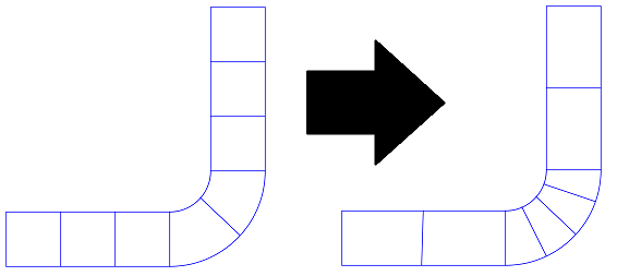
r-refinement is the modification of mesh resolution without changing the number of nodes or cells present in a mesh or the connectivity of a mesh. The increase in resolution is made by moving the grid points into regions of activity, which results in a greater clustering of points in those regions. The movement of the nodes can be controlled in various ways. On common technique is to treat the mesh as if it is an elastic solid and solve a system equations (suject to some forcing) that deforms the original mesh (see for instance Stretched grid method). Care must be taken, however, that no problems due to excessive grid skewness arise.
h-Refinement
h-refinement is the modification of mesh resolution by changing the mesh connectivity. Depending upon the technique used, this may not result in a change in the overall number of grid cells or grid points. The simplest strategy for this type of refinement subdivides cells, while more complex procedures may insert or remove nodes (or cells) to change the overall mesh topology.
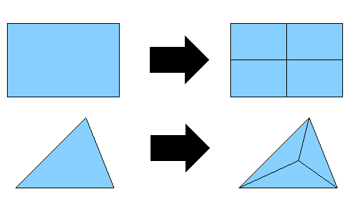
In the subdivision case, every "parent cell" is divided into "child cells". The choice of which cells are to be divided is addressed below. For every parent cell, a new point is added on each face. For 2-D quadrilaterals, a new point is added at the cell centroid also. On joining these points, we get 4 new "child cells". Thus, every quad parent gives rise to four new offsprings. The advantage of such a procedure is that the overall mesh topology remains the same (with the child cells taking the place of the parent cell in the connectivity arrangement). The subdivision process is similar for a triangular parent cell, as shown below. It is easy to see that the subdivision process increases both the number of points and the number of cells.
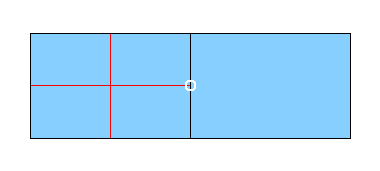
An additional point to be noted is that this type of mesh adaptation can lead to what are called "hanging nodes." In 2D, this happens when one of the cells sharing a face is divided and the other is not, as shown below. For two quad cells, one cell is divided into four quads and other remains as it is. The highlighted node is the hanging node.
This leads to a node on the face between the two cells which does not belong (properly) to both of the cells. The node "hangs" on the face, and one of the cells becomes an arbitrary polyhedron. In the above case, the topology seemingly remains same, but the right (undivided) cell actually has five faces.
Further, there are two ways of h-refinement: Isotropic and Anisotropic. Isotropic refinement, is what was described a little back. In isotropic refinement, new points are added in both the directions, say x and y. In anisotropic refinement, the division takes place in one predominant direction. Thus, in short, an isotropic refinement for a quad would produce four new offsprings, while anisotropic refinement would only generate two. Anisotropic refinement is made use of, when the user knows that the flow feature is predominantly to be resolved in one direction, for e.g. Boundary Layers. However, there are situations where an anisotropic refinement alone may not be satisfactory, such as a shock-boundary layer interaction.
The simplest reifnement anyone can think of is to divide all cells in the domain. This is referred to as "Uniform Refinement". Although it does improve the solution vastly, it is easy to realise that we are going for a huge unwanted effort in doing so. For e.g., in the farfield region of an airfoil, cell division is not bringing in any improvement because the flow there does not experience any activity. Therefore, to achieve the goal of mesh adaptation, the refinement is done at "selected" regions alone based on certain criterion. This is referred to popularly as AMR or Adaptive Mesh Refinement. It is to be remarked that AMR does not only encompass division of cells into smaller ones ( Refinement ), but also the agglomeration of smaller cells into a larger one (De-refinement or coarsening), when the need arises.
p-Refinement
A very popular tool in Finite Element Modelling (FEM) rather than in Finite Volume Modelling (FVM), it achieves increased resolution by increasing the order of accuracy of the polynomial in each element (or cell).
In AMR, the selction of "parent cells" to be divided is made on the basis of regions where there is appreciable flow activity. It is well known that in compressible flows, the major features would include Shocks, Boundary Layers and Shear Layers, Vortex flows, Mach Stem , Expansion fans and the like. It can also be seen that each feature has some "physical signature" that can be numerically exploited. For eg. shocks always involve a density/pressure jump and can be detected by their gradients, whereas boundary layers are always associated with rotationality and hence can be detected using curl of velocity. In compressible flows, the velocity divergence, which is a measure of compressiblity is also a good choice for shocks and expansions. These sensing paramters which can indicate regions of flow where there are activity are referred to as ERROR INDICATORS and are very popular in AMR for CFD.
Just as refinement is possible by ERROR INDICATORS as mentioned above, certain other issues also assume relevance. Error Indicators do detect regions for refinement, they do not actually tell if the resolution is good enough at any given time. In fact the issue is very severe for shocks, the smaller the cell, the higher the gradient and the indicator would keep on picking the region, unless a threshold value is provided. Further, many users make use of conservative values while refining a domain and generally end up in refining more than the essential portion of the grid, though not the complete domain. These refined regions are unneccesary and are in strictest sense, contribute to unneccesary computational effort. It is at this juncture, that reliable and resonable measure of cell error become necessary to do the process of "coarsening", which would reduce the above-said unnecessary refinement, with a view towards generatin an "optimal mesh". The measures are given by sensors referred to as ERROR ESTIMATORS, literature on which is in abandunce in FEM, though these are very rare in FVM.
Control of the refinement and/or coarsening via the error indicators is often undertaken by using either the 'solution gradient' or 'soultion curvature'. Hence the refinement variable coupled with the refinement method and its limits all need to be considered when applying mesh adaptation.
<< Unstructured Mesh Generation | Mesh Adaptation | First cell height calculation>>


